ggplot and concepts -- what's right, and what's wrong

The ggplot package, written by the overachieving and remarkable Hadley Wickham, is based on earlier more theoretical work by Leland Wilkinson. Wilkinson abstracted the process of putting data onto an image, and created a Grammar of Graphics, which describes how the data maps to the parts of a graph, rather than describing the final graph itself. For example, here’s how to create a pie chart, clipped from Wilkinson’s book:

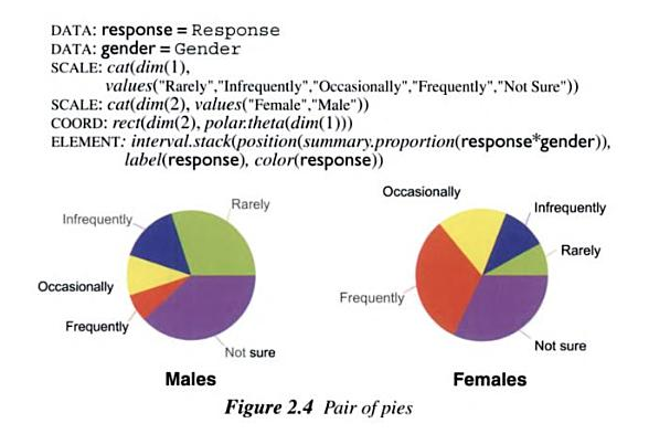
Don’t worry about the details, but briefly, a pie chart is just a stacked bar graph (summary.proportion) plotted in polar coordinates (polar.theta). If you took the time to learn this grammar, you would realize that the hierarchical structure of a graph on a page (elements have positions and labels and visual properties like color, each of which have their own abstract structure) maps cleanly to the hierarchical structure of the grammar, and that variables in the grammar map cleanly to the linear structure of the data. As a user of this system, you would be able to see all three key representations at once: the data, the grammatical mapping from data to graph, and the graph itself.

Now consider ggplot, the implementation of the Grammar of Graphics in the R programming language. Does ggplot maintain three visible representations, all straightforwardly mappable to each other? Sadly, it does not. Instead, users of ggplot must map among four representations: the data (a standard data.frame object), the R syntax for ggplot2 (which has some quirks), an underlying ggplot object (similar to the Grammar of Graphics, but vastly more complex and impossible to examine directly), and the generated graph.

Consider the simple pie graph, below.

This chart is generated in ggplot2 by the following R code:

> zz <- data.frame(cat=c("a", "b"), val=c(5,3))

> zz
 cat val
1   a   5
2   b   3
> pp <- ggplot(zz, aes(x="", y=val, fill=cat)) + geom_bar(width=1) + 
        coord_polar("y")
> print(pp)

The print() function is optional within an R interpreter session, but I include because it illustrates a point that’s not initially obvious to many users. Unlike the built-in R plotting tools, the ggplot() function and its associated functions don’t plot anything on the screen, they just construct an object of type “ggplot”. Almost all of the actual work of mapping the data to stuff on your screen occurs when you print that object, using print() or ggsave().

So what does that object look like? If you type str(pp), you’ll get an answer, but it’s about a hundred lines of undecipherable hierarchical object and list structure, not intended to be examined by mere mortals. But there’s something critically important about that structure – like the original Grammar of Graphics, and unlike the R syntax above, it’s hierarchically structured.

In the R syntax, you create a base ggplot structure with the ggplot() call, then you abuse the “+” operator to make changes to that structure. The geom_bar() function adds a layer to the ggplot() object, where a layer is just what it sounds like, a set of information about one of potentially many overlaid layers of content that will be put on the graph. So you construct a ggplot object by first initializing everything about the basic plot, then tack on layers with +, right? Actually no, because the coord_polar() call doesn’t create or modify a layer at all, it modifies the base object! Even if you’ve acquired the nonobvious intuition that ggplot objects are hierarchical and are created by concatenating layers, you now have to break the analogy again to fully understand what + is doing!

There is a way to partially see the structure directly, but it’s not well thought-out from the point of view of someone trying to learn how to use the package. The summary() method on ggplot objects tells you about things you didn’t specify (faceting?), it’s incomplete, and it doesn’t map well to the R syntax. If something in your plot isn’t working the way you want it to, summary() won’t help you.

> summary(pp)
mapping:  x = , y = val, fill = cat
faceting: facet_grid(. ~ ., FALSE)
-----------------------------------
geom_bar:
stat_bin: width = 1
position_stack: (width = NULL, height = NULL)

Another shortcut that leads to conceptual problems by ggplot beginners is the use of qplot(). The qplot() function is a wrapper around ggplot(). Unlike ggplot(), you can give qplot() data that is not in the form of a data.frame, and the syntax is somewhat different. There’s nothing wrong with some syntactic sugar to make life easier, but in this case, learning ggplot by starting with qplot is like trying to learn a foreign language by starting with contractions and slang. You may be able to say a few essential things on your vacation, but you won’t be able to creatively construct new sentences as new situations arise. The brilliance of the Grammar of Graphics is exactly that it’s a grammar – you can construct new graphs and new types of graphs as new situations arise! But tutorials that start with qplot, with the ggplot book an unfortunate (but in other ways excellent) example, send their learners down a linguistic garden path. To fully use the power of the system requires unlearning the conceptual structures that map the slang to charts on a screen, and starting over with learning the new, more powerful ggplot() grammar and hierarchical representations.

I’d like to conclude this overlong rant with two notes. First, just today a new graphics package for R was introduced. jjplot uses many of the ideas of the Grammar of Graphics and ggplot2, but seems to avoid at least a few of the conceptual problems. The + operator is not overloaded in conceptually confusing ways, and there is no distracting qplot function to mislead new users. Additionally, a quick look at the source code finds it much, much simpler than ggplot2’s source, which will likely lead to a more active base of contributors. I look forward to trying jjplot and watching its continuing development, and hope the authors learn from both the remarkable successes and frustrating failures of ggplot. Second, I use ggplot extensively in my work. It’s simply the best available tool for quickly generating elegant graphs of data in R, especially if that generation needs to happen automatically in code. Hadley Wickham deserves extensive praise for the amount of effort he has put into developing and popularizing the Grammar of Graphics. If you want to be maximally effective when visualizing data in R, take the time to learn ggplot2, but do so while keeping in mind that the learning process will be easiest if you skip qplot and other shortcuts, think hierarchically, and prepare for some frustration. Fortunately, the support communities on the ggplot mailing list and Stack Overflow are extremely helpful, as is Hadley himself.